Applications & Software
This page presents software and computational material developed in connection with the research activities of the Actuarial-Financial Mathematics Lab. The emphasis is placed on mathematically grounded methods for portfolio construction, derivative valuation, risk analysis, and stochastic modelling, together with Python implementations that support both research and teaching.
A central objective of our work is to study how optimization methods, option contracts, and stochastic models can be used in a coherent framework for decision-making under uncertainty. In this context, portfolio construction is viewed not only as a numerical problem, but also as a problem of mathematical modelling in which the available financial instruments, the market data, and the investor's assumptions all play a significant role.
In parallel, we develop software that illustrates the mathematical structure of these problems and allows the user to experiment with real or historical data. The corresponding codes are intended both as computational tools and as educational resources that make the underlying theory more transparent.
Development of Software with Practical and Educational Interest
Our goal is to develop software that combines mathematical rigor with practical relevance. The following projects represent some of the directions in which this work is currently being developed.
-
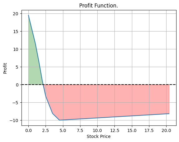
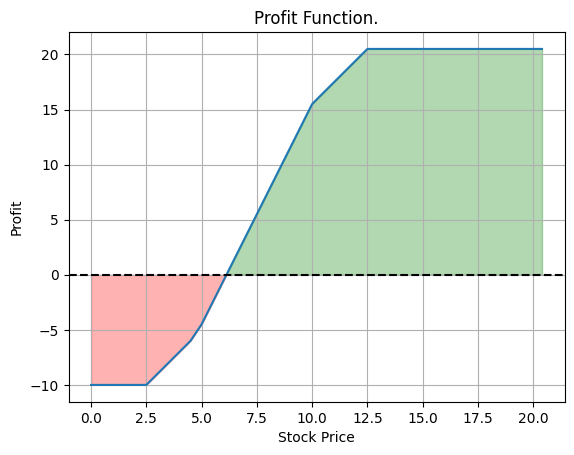
Given a forecast for the future value of a stock, one may enrich a portfolio with suitable call and put options in order to obtain a prescribed profit profile under the anticipated market scenario. This approach leads naturally to an optimization problem in which the available contracts and their bid-ask spreads are explicitly taken into account. The figure below illustrates such a construction based on real market data. The corresponding implementation is available in the following Python package: Portfolio construction with calls and puts . The same material also includes code for detecting possible arbitrage opportunities when a stock and the associated call and put options are given.
-
Classical portfolio theory is typically formulated in terms of historical returns, variances, and covariances. Within this framework, the construction of an efficient portfolio depends strongly on the quality of the forecasting stage. Our work aims to refine the portfolio-construction stage by incorporating a broader class of available financial instruments, while leaving open the complementary challenge of improving the forecasting stage through machine learning and artificial intelligence.
-
We have also developed Python code for the implementation of Markowitz portfolio optimization for an arbitrary number of stocks. The code uses historical market data in order to estimate variances and covariances and to construct admissible portfolios: Markowitz Portfolio Construction .
-
Source code and supplementary computational material are also available through our GitHub repository: GitHub Repository .
-
Additional notes and supporting documentation may be downloaded here: Supplementary PDF Material .
Sample Computational Output
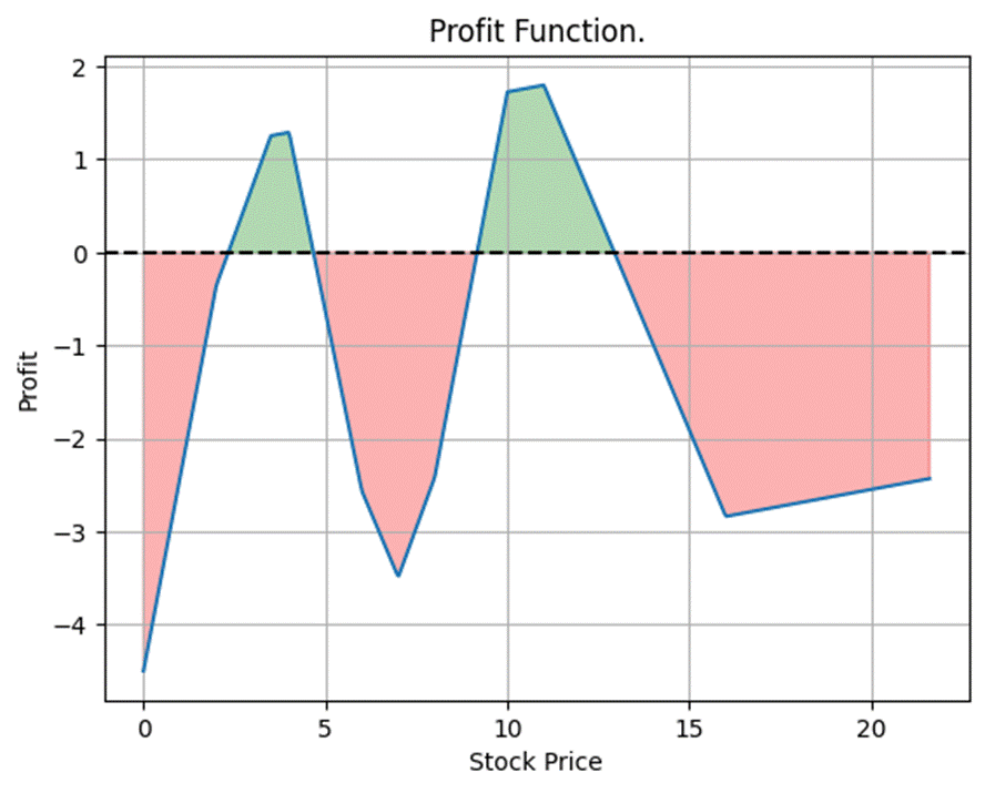
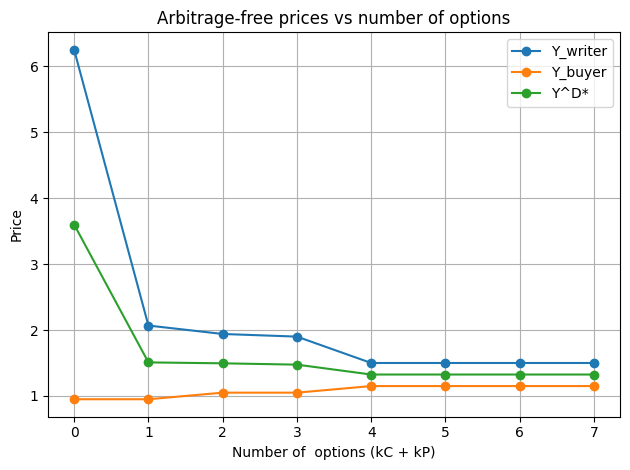
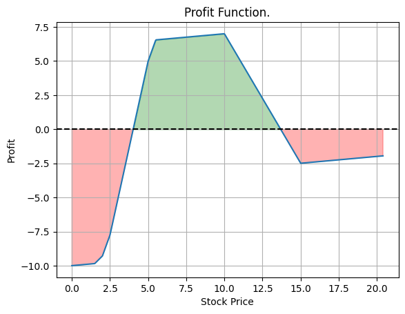
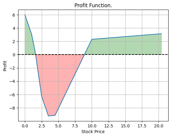
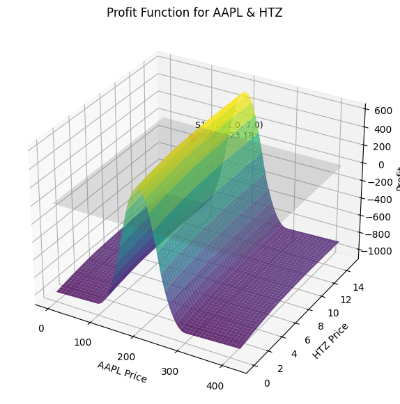
The following figures present indicative computational output from our Python implementations, including profit functions, arbitrage-free price intervals, and multi-asset payoff surfaces. We observe that the profit function can be sculpted in an arbitrary manner through the use of options. Our methodology includes all standard option strategies, such as butterfly spreads and similar constructions. Furthermore, in the figure where the arbitrage-free interval is seen to contract as more options are added, it becomes clear that this leads to a more precise target price for a new option whenever we require its value to remain arbitrage-free.
-
For the valuation of derivative contracts, we have developed Python code that computes arbitrage-free price intervals for contracts with user-defined payoff functions, under appropriate structural assumptions. In particular, the code can be used for piecewise linear payoff functions with finitely many branches and can be applied using real market data, including bid-ask spreads. This framework is intended as a flexible computational environment for the study of derivative valuation in the presence of traded options.
The relevant implementations are included in the corresponding package, where one may also find auxiliary tools for writer and buyer hedging strategies. In addition, we provide codes for more classical valuation models based on historical volatility estimates: Black-Scholes Fair Price and Binomial Model .
-
Another important topic in financial mathematics is dynamic trading. We study trading rules that depend on the evolution of the stock price and on assumptions concerning future fluctuations. This leads naturally to stochastic modelling and to the numerical approximation of continuous-time processes. Our broader objective is to develop code that assists in the identification of suitable dynamic trading strategies within mathematically well-defined frameworks.
More generally, a natural continuation of this work is the study of portfolios containing several stocks together with derivative contracts, as well as forecasting techniques capable of incorporating not only historical numerical data but also recent events and cross-asset dependencies.
It is important to distinguish between forecasting and optimization. In portfolio construction and dynamic trading, a forecast or market scenario is typically part of the input. By contrast, in derivative valuation problems formulated in terms of no-arbitrage principles, the mathematical aim is usually to identify admissible price ranges or hedging structures that are consistent with the available market information.
Users of the software are encouraged to verify the resulting profit functions independently and to interpret the numerical output together with the assumptions under which it has been derived. In particular, all calculations should be understood relative to the quality of the data, the modelling hypotheses, and the actual execution prices available in the market.
-
In the Python code Geometric Brownian Motion and Applications , one can estimate the parameters μ and σ under the assumption that the stock price follows geometric Brownian motion, using historical data obtained from Yahoo Finance. The code can then be used to compute probabilities associated with future price intervals, including the probability of an increase in value. Such results may serve as model-based forecasts, which can subsequently be combined with the portfolio-construction tools described above. At the same time, it should be emphasized that conclusions derived from a prescribed probabilistic model remain dependent on the validity of the corresponding modelling assumptions.